import plotly.graph_objects as go

# Define the data
labels = [
    "Energy",
    "Generation", "Storage", "Transmission",
    "Fossil", "Renewable", "Nuclear",
    "Short-term", "Long-term",
    "Grid Infrastructure", "Efficiency", "Energy Conversion",
    "Solar", "Wind", "Hydro", "geothermal", "biomass", "tidal",
    "Oil","Gas","Coal",
    "Lithium-ion batteries", "Supercapacitors", "Pumped hydro storage", "Compressed Air Energy Storage",
    "Hydrogen storage", "Flow batteries", "Power-to-Gas", "Cryogenic energy storage",
]

parents = [
    "",
    "Energy", "Energy", "Energy",
    "Generation", "Generation", "Generation",
    "Storage", "Storage",
    "Transmission", "Transmission", "Transmission",
    "Renewable", "Renewable", "Renewable", "Renewable", "Renewable", "Renewable",
    "Fossil","Fossil","Fossil",
    "Short-term", "Short-term", "Short-term", "Short-term",
    "Long-term", "Long-term", "Long-term", "Long-term"
]

# Update values to represent market share (these are example values, adjust as needed)
values = [
    100,  # Energy (total)
    69, 30, 1,  # Generation, Storage, Transmission
    65, 27, 8,  # Fossil, Renewable, Nuclear
    12.5, 37.5,  # Short-term, Long-term
    7, 2.5, 2.5,  # Grid Infrastructure, Efficiency, Energy Conversion
    16, 20, 40, 8, 15, 1,  # Solar, Wind, Hydro, Geothermal, Biomass, Tidal
    25, 35, 45,  # Oil, Gas, Coal
    38.5, 1.5, 12.5, 2.5,  # Lithium-ion, Supercapacitors, Pumped hydro, Compressed Air
    22.5, 12.5, 12.5, 2.5,  # Hydrogen, Flow batteries, Power-to-Gas, Cryogenic
]

# Create the sunburst chart
fig = go.Figure(go.Sunburst(
    labels=labels,
    parents=parents,
    values=values,
))

# Update the layout
fig.update_layout(
    title="Energy Sector Sunburst Chart",
    width=800,
    height=800,
)

# Show the chart
fig.show()Understanding Energy Sub-Sectors: Part 1
energy
ai
series
Article Summary
Understand the energy market’s sub-sectors and how the market as a whole connects together
Mapping out the energy space
A quick foreword—I’m an AI guy and I use it for lots of things.
While I don’t like to use it for writing, as it tends to create voiceless and untrustworthy text, it does one thing REALLY well….

Claude helped me to brainstorm the list (which I heavily curated and modified) that I’m using as my roadmap for understanding the energy market as a whole.
Why did I write this?
The AI world has a lot of mania at the time of this writing, and as a “career AI guy,” it is essential to understand the underlying forces that help drive (or kill 💀) the growth of the AI bubble.
Alongside the mega-minds and hype men, the AI industry requires many ingredients such as computational power, infrastructure capabilities, and power generation.
I don’t know much about how the energy space works as a whole, but I do know that AI requires a lot of it. How much specifically?
AI servers could use 0.5% of the world’s electrical generation by 2027. For context, data centers currently use around 1% of global electrical generation… this suggests an electricity consumption of approximately 3 Wh per LLM interaction.
Cell Press. (2023). Joule, Volume 7, Issue 7. Retrieved from https://www.cell.com/joule/fulltext/S2542-4351(23)00365-3
While writing this article, I made at least 100 LLM interactions, using about 300 Wh, so for context my AI usage was about the equivalent to a 10-watt LED light bulb running for 30 hours.
Most importantly—I can’t fix a problem that spans such a wide range of areas. Focusing on a specific issue in a specific industry could lead to a solvable stepping stone and better understanding the market forces as a whole!
Understanding the energy sub-sectors and breaking them down into clusters
I’m currently clustering sub-sectors into three primary categories:
- energy generation ($4-5 trillion market cap)
- Fossil Fuels: ~110,500 TWh (65%)
- Coal: ~44,200 TWh (40% of fossil fuels)
- Natural Gas: ~38,675 TWh (35% of fossil fuels)
- Oil: ~27,625 TWh (25% of fossil fuels)
- Renewable Energy: ~46,000 TWh (27%)
- Hydropower: ~18,400 TWh (40% of renewables)
- Wind: ~9,200 TWh (20% of renewables)
- Solar: ~7,360 TWh (16% of renewables)
- Biomass: ~6,900 TWh (15% of renewables)
- Geothermal: ~3,680 TWh (8% of renewables)
- Tidal/Wave: ~460 TWh (1% of renewables)
- Nuclear Energy: ~13,500 TWh (8%)
- Fossil Fuels: ~110,500 TWh (65%)
- energy storage ($2-3 trillion market cap)
- short-term storage solutions ($350-400 billion market cap)
- long-term storage solutions ($150-200 billion market cap)
- energy transmission ($50-100 billion market cap)
The following have been grouped into tangential categories with significant influence on the energy space as a whole:
- energy markets and trading
- energy policy and regulation:
- energy data and analytics:
- sustainability and environmental impact:
This follows a relatively intuitive flow: man generates energy → man stores some of that energy → man moves around and uses some of that energy.
I’ll outline the roadmap in this article and then delve into each of the sub-sectors in separate articles, as each represents multiple billion-dollar industries.
For example, the energy generation sub-sector includes fuel sources, methods of refinement, and utilization per fuel source (too much to detail here).
The following diagram represents the three primary categories defined above in a sunburst chart, with the size of each chunk representing its market cap relative to the energy space as a whole (roughly estimated to be seven trillion dollars for this example).
The final child nodes of the sunburst were calculated by estimating how much of the global 170,000 TWh (terawatt-hours) each energy source contributed.
I’ll be focusing on the tangential markets in a later post.
Initial takeaways
I was surprised to see that energy generation had such a large share of the over all energy market. It makes intuitive sense that resources used to produce energy would play a substantial role, but I didn’t anticipate that the majority of energy would be utilized (or perhaps lost) before storage and transmission played a bigger role.
- note to self for future investigation 🕵️♂️—better understand how much energy gets lost before it even leaves the building…
Hydro energy being the largest of the renewables by a significant factor was also surprising. Regions of the country with large rivers and waterfalls produce disproportionate amounts of energy to their usage!
I also had no idea that you could store energy by essentially pumping / compression resources such as water and air for future kinetic gains (a spicy physics trick 🌶️).
I’d like to see how market growth in each sector compares to one another to better understand what has potential for expansion and which has stagnated. Energy policy plays a large role in what wins and what loses.
At least I now have a general understanding, if imperfect, on how the forces of the market interact and their relative sizes.
I will now begin the deep dive into each slice of the sunburst chart to get a sense for how that process works, where it falls short, and the innovations / initiatives going on it to piggy back off.
If I had to throw a dart at the dartboard to understand where AI could play a role in energy, I’d land on the following:
Areas immediately jumping out that AI can assist in:
- grid management
- optimizing mixed storage types and methods for grid utilization
- improvements to energy methods
- Predictive modeling for optimal charge/discharge cycles
- energy efficiency optimizations
- industrial process energy efficiency
- Developing smart control systems for buildings and appliances
- general energy conversions / generation AI modeling
- Optimization of storage system operations
- predictive maintenance
- predictive modeling of energy consumption patterns (storage and conversion impacts)
- market forecasting
Not too imaginative or specific yet! I tend to imagine AI as the ultimate prediction tool that can find ways to move molecules from point A to point B in unexpected ways.
Defining a bandit
A bandit represents an environment, a set of rewards, and a set of actions.
For example, a one armed bandit has one possible action (one “arm” or lever) in its environment and pulling that arm generates one set of rewards–typically as a randomly generated number between two set intervals such as 0 and 1.
Why bandits?
RL agents use evaluation methods to dictate what actions it takes, instead of instruction from a combination of loss/reward/etc. functions.
Guiding an RL agent through evaluative feedback will help it understand which actions provide the most reward but doesn’t specify which action provides the best or worst outcomes.
Bandits allow us to create simple test beds for training RL agents in. An RL agent must learn to maximize total reward when interacting with the bandit given a number of action selections.
If your bandit has three arms and the RL agent can choose to pull one of those three levers 1000 times–which combination of lever pulls will lead to the highest possible reward? An effective RL agent should learn the optimal sequence of when and which levers to pull.
Providing bandit actions a value
In life and in RL, if we had a perfect understanding of the short and long term value tied to an action we would be able to exploit that to our advantage.
Let’s create some perfect ground truth values for a three armed bandit.
import numpy as np
import matplotlib.pyplot as plt

# assign a random starting seed value
np.random.seed(5)

# basis for generating the reward ground truths
mean = 0          # also known as mu
standard_deviation = 1      # also known as sigma
arms = 3

# bandit values
action_range = np.arange(0, arms)
reward_truths = np.random.normal(mean, standard_deviation, (arms))
total_actions_allowed = 1000

# plot initial ground truth values
plt.plot(action_range, reward_truths, 'o', color='black')

# plot details
plt.xlabel('Arm Number')
plt.ylabel('Arm Value')
plt.xticks(range(0,arms))
plt.title('Initial Bandit Arm Ground Truth Values')
plt.show()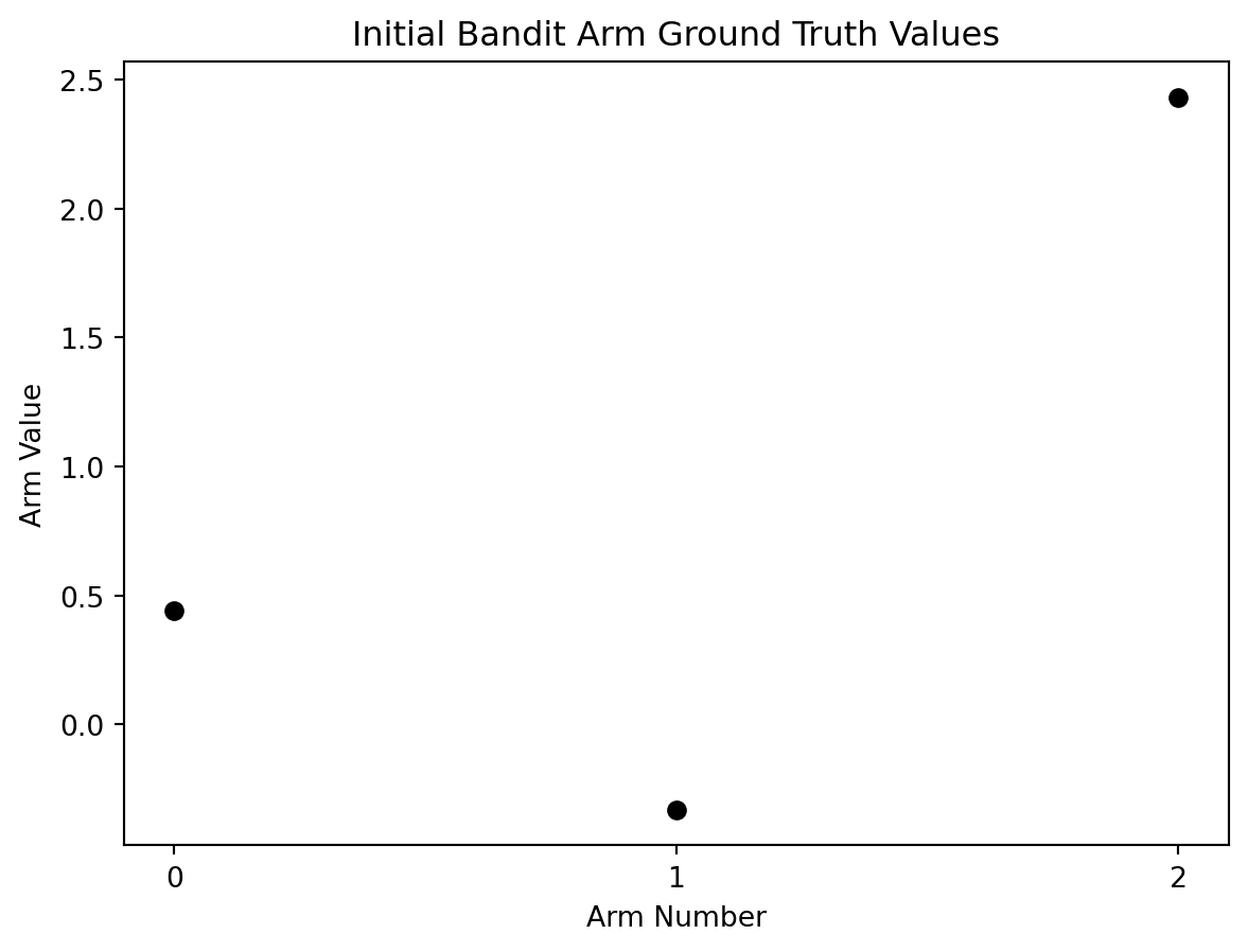
Unfortunately, we don’t have perfect knowledge so we as agents must do our best to estimate the reward value of an action before we take it.
We can’t provide a static ground truth value for a bandit arm or else a greedy RL agent will always be able to quickly solve the problem in a way that doesn’t replicate real world situations.
A better action-value method
A good bandit arm should be assigned a set reward value to act as the ground truth, a range of possible reward values to pull from anchored on the ground truth, and the resulting reward should be randomly sampled from that range when the arm gets pulled.
I like to think of this as applying a standard deviation error bar to your starting point.
# apply a standard deviation error bar to the ground truth values
plt.errorbar(action_range, reward_truths, np.ones(arms), fmt='o')

# plot details
plt.xlabel('Arm Number')
plt.ylabel('Arm Value')
plt.xticks(range(0,arms))
plt.title('Initial Bandit Arm Ground Truth Values with Deviation Range')
plt.show()

plt.show()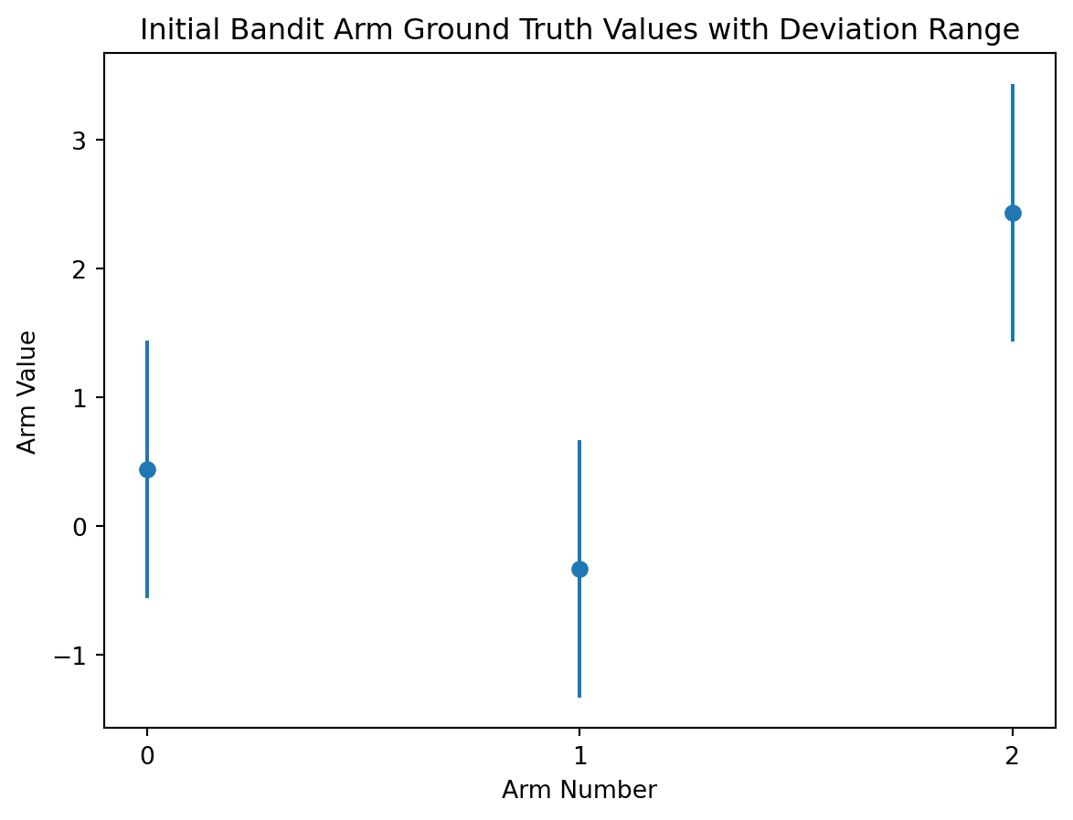
In implementation, the agent will use a properly sampled distribution of actions and not a deviation bar.
Let’s update the the visualization of each bandit arm with 1000 sampled data points to better capture these good practices.
# for each arm's reward truth, generate distribution between 1 and total_actions_allowed
reward_ranges = np.array([np.random.normal(true_reward,1,total_actions_allowed) for true_reward in reward_truths])

# plot scatter points representing the sampled value range centered on ground truth value
for i in action_range:
    plt.scatter(np.full((total_actions_allowed),i),reward_ranges[i])

# plot ground truth ranges
plt.plot(action_range, reward_truths,'o', color='black')
plt.xlabel('Arm Number')
plt.ylabel('Arm Value')
plt.xticks(range(0,arms))
plt.title('Initial Bandit Arm Ground Truth Values with Sampling Applied')
plt.show()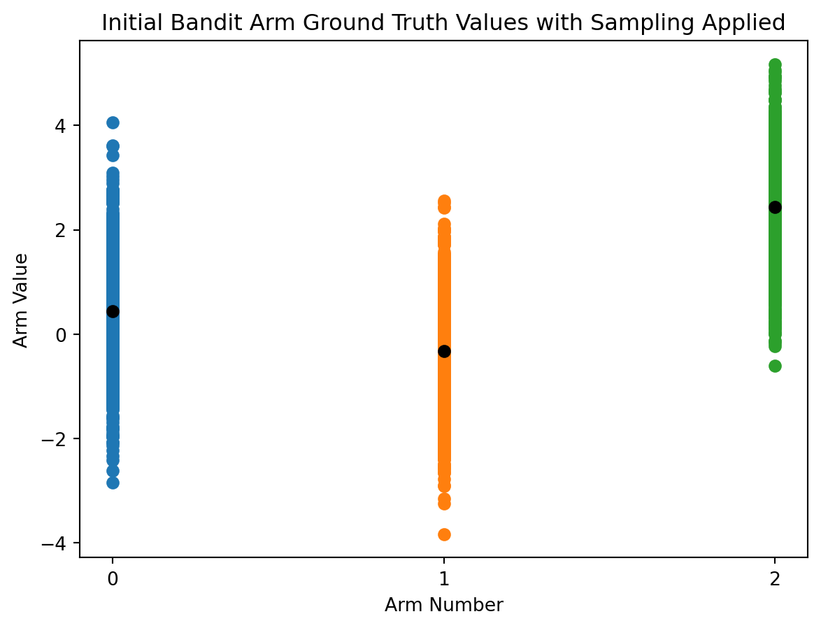
For each additional bandit arm we add, the same process will occur. Check out a 15 arm bandit, with twice the standard deviation, that has 2000 total action “time steps”.
# updated bandit values
arms = 15
standard_deviation = 2
action_range = np.arange(0, arms)
reward_truths = np.random.normal(mean, standard_deviation, (arms))
total_actions_allowed = 2000

# for each arm's reward truth, generate distribution between 1 and total_actions_allowed
reward_ranges = np.array([np.random.normal(true_reward,1,total_actions_allowed) for true_reward in reward_truths])

# plot scatter points representing the sampled value range centered on ground truth value
for i in action_range:
    plt.scatter(np.full((total_actions_allowed),i),reward_ranges[i])

# plot ground truth ranges
plt.plot(action_range, reward_truths,'o', color='black')
plt.xlabel('Arm Number')
plt.ylabel('Arm Value')
plt.xticks(range(0,arms))
plt.title('Initial Bandit Arm Ground Truth Values with Sampling Applied')
plt.show()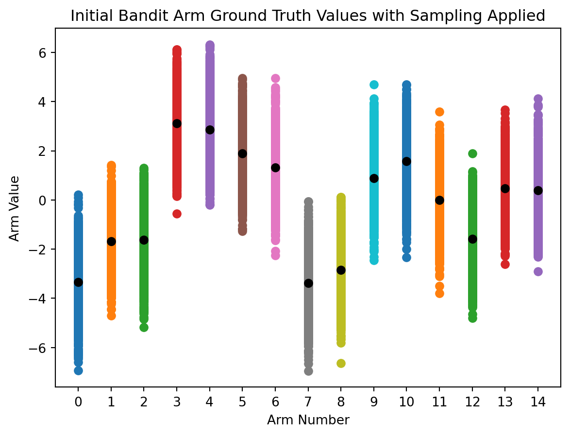
The wider range of values to sample from and increased number of arms increase the complexity, thereby making it harder for the agent to find the optimal value function.
Next up
Now that we know how to create a simple n-armed bandit, we need to build an RL agent capable of maximizing reward during interactions.
Link will be updated here when complete!